BMN(Boundary-Matching Network) 详解。
Intro
百度,ActivityNet Challenge 2019 冠军模型:BMN: Boundary-Matching Network for Temporal Action Proposal Generation。
Problem Formulation
- Unlike temporal action detection task, in the work categories of action instances are not taken into account in proposal generation task.
- The temporal annotation: $\Psig=\left { \varphi_n=(t{s,n}, t{e,n}) \right } ^{N_g}{n=1}$, here $N_g$ is the amount of ground-truth action instances.
- During inference, proposal generation method should generate proposals $\Psi_p$ which cover $\Psi_g$ precisely and exhaustively.
网络结构:
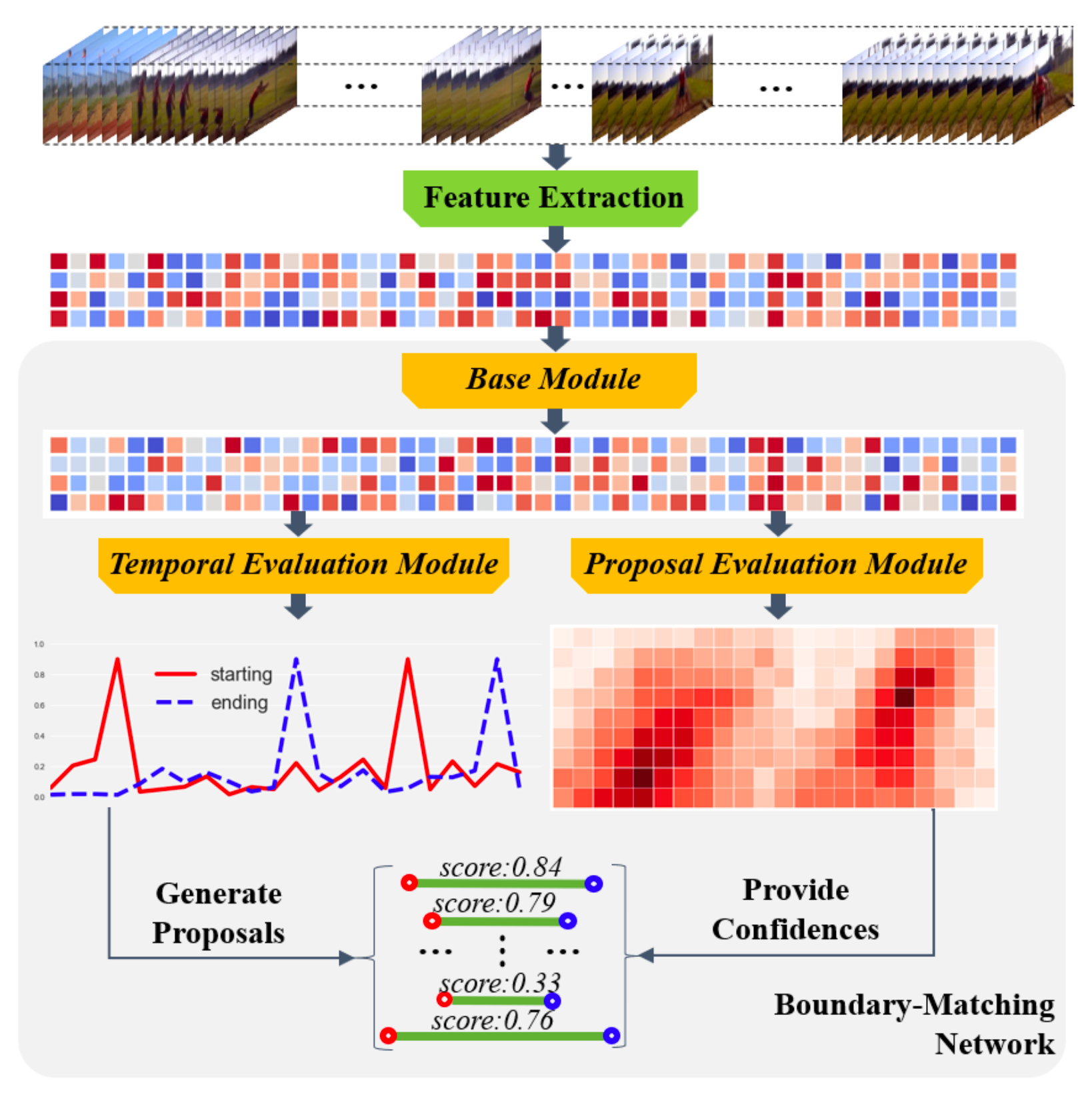
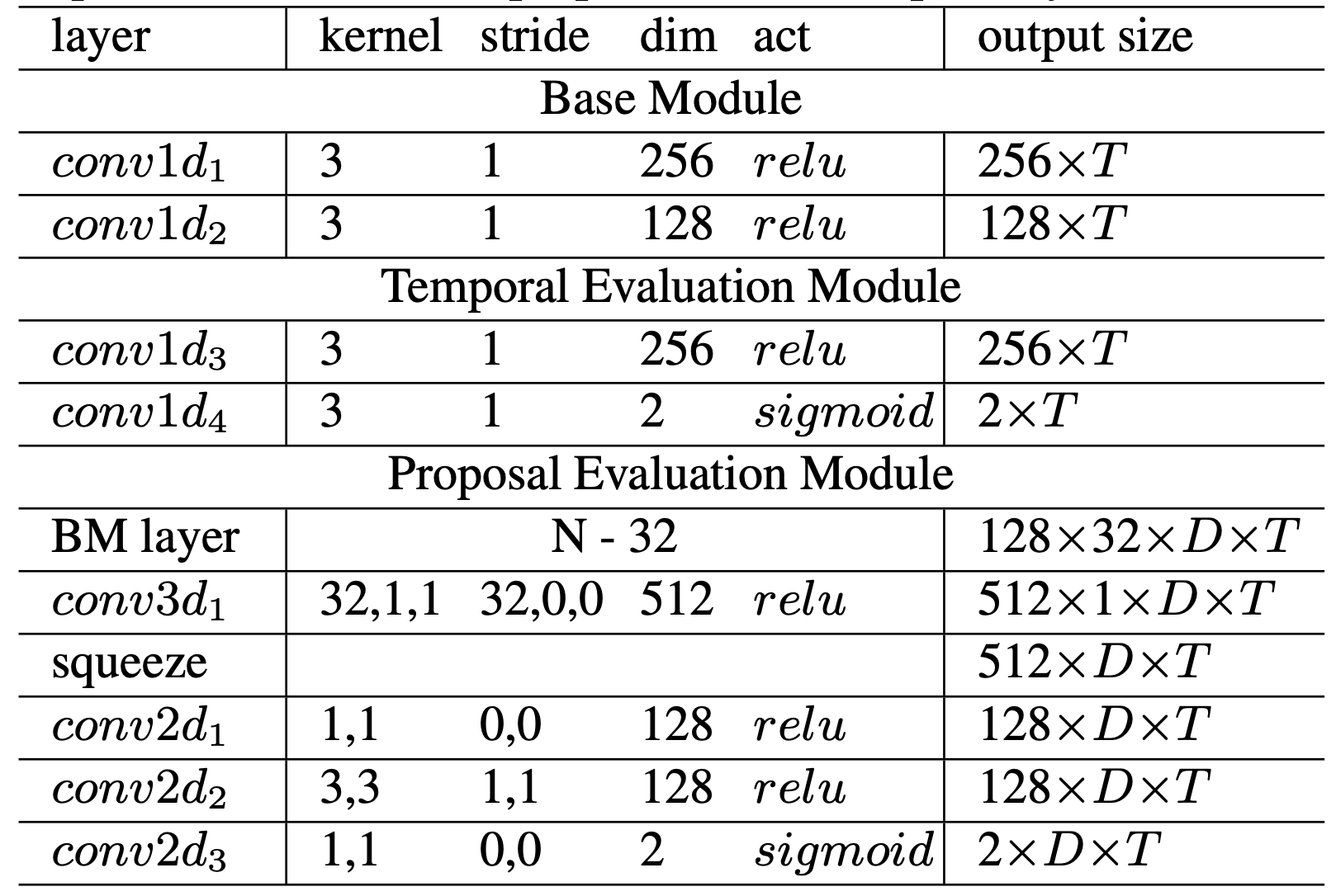
流程
- Feature Extraction: 使用双流网络(光流+RGB),获得feature map.
- Base Module: 1x1卷积(时序卷积)。
- Temporal Evaluation Module(TEM): 1x1卷积(时序卷积),获得开始、结束点的概率序列。
- Proposal Evaluation Module(PEM):
- [[PapersRead#BMN#BM layer|BM layer]]
- 通过conv3d, conv2d 得到置信度图。
- 生成结果:
- 把两条边界概率序列中大于$极大值\times \frac{1}{2}$ 或是峰值(极大值)的都看作开始或结束边界.
- $n^2$复杂度两两组合,获得一系列proposals:
- 根据置信度图获得各个proposals的置信度。
- the proposal denoted: $φ = (ts, t_e, p^s{ts} , p^e{te} , p{cc}, p{cr})$
where $p^s{ts}, p^e{te}$ are starting and ending probabilities. $p{cc}, p_{cr}$ are classification confidence and regression confidence score. - get final score: $pf = p^s{ts} · p^e{te} · \sqrt{p{cc}· p_{cr})}$
- the proposal denoted: $φ = (ts, t_e, p^s{ts} , p^e{te} , p{cc}, p{cr})$
- 利用Soft-NMS去冗余。
置信度图:
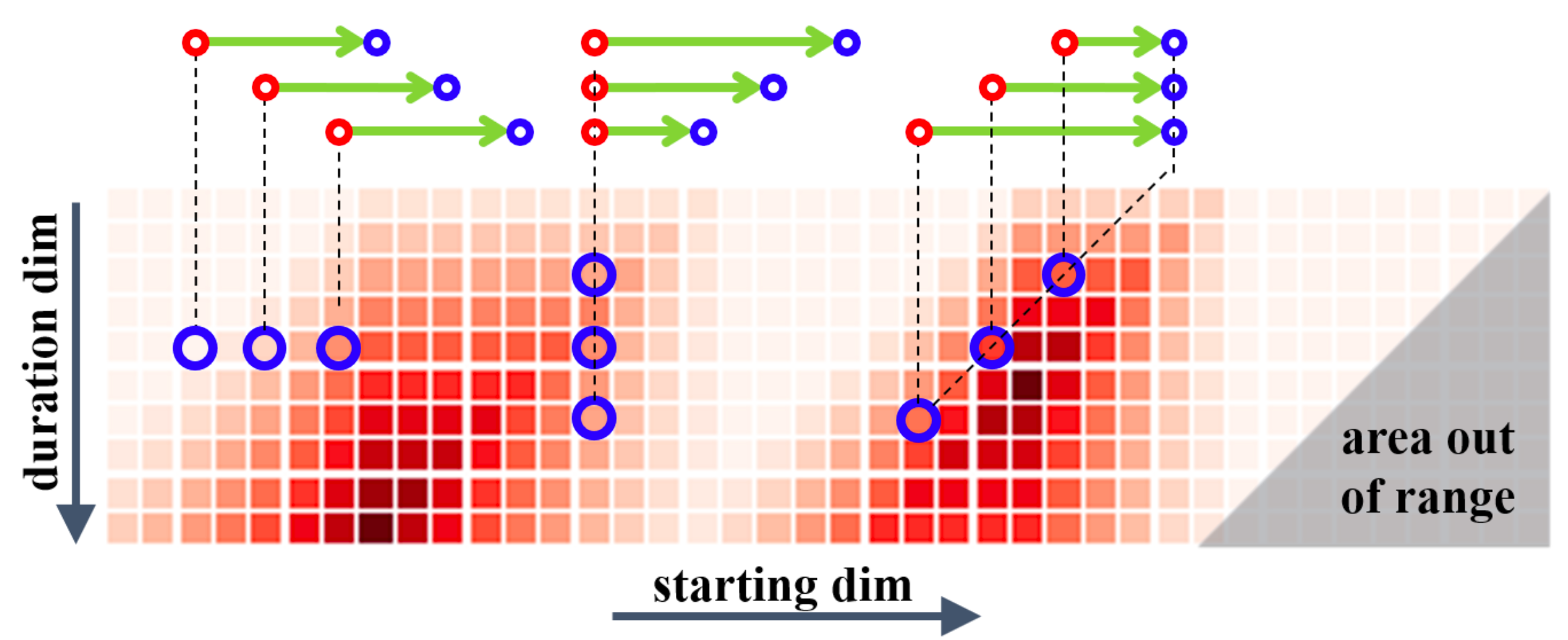
- $M_C\in R^{D×T}$.
- 由开始点和长度决定结束点,从而确定一个proposal. 所以上图对应所有任意视频段的置信度。
- duration dim: proposal长度.
- starting dim: 开始点位置。
- 同一行对应的proposals对应相同的长度。同一列队对应的proposals拥有相同的开始点。同一负对角线对应的proposals拥有相同的结束边界。右下角部分proposals超出视频范围,无意义。
BM layer
- The goal: uniformly sample N points in $S{F} ∈ R^{C×T}$ between starting boundary $t{s}$ and ending boundary $t{e}$ of each proposal $φ{i,j}$, and get proposal feature $m^f_{i,j} ∈ R^{C×N}$ with rich context (actually sampling in [$t_S-0.25d, t_e+0.25d$]).
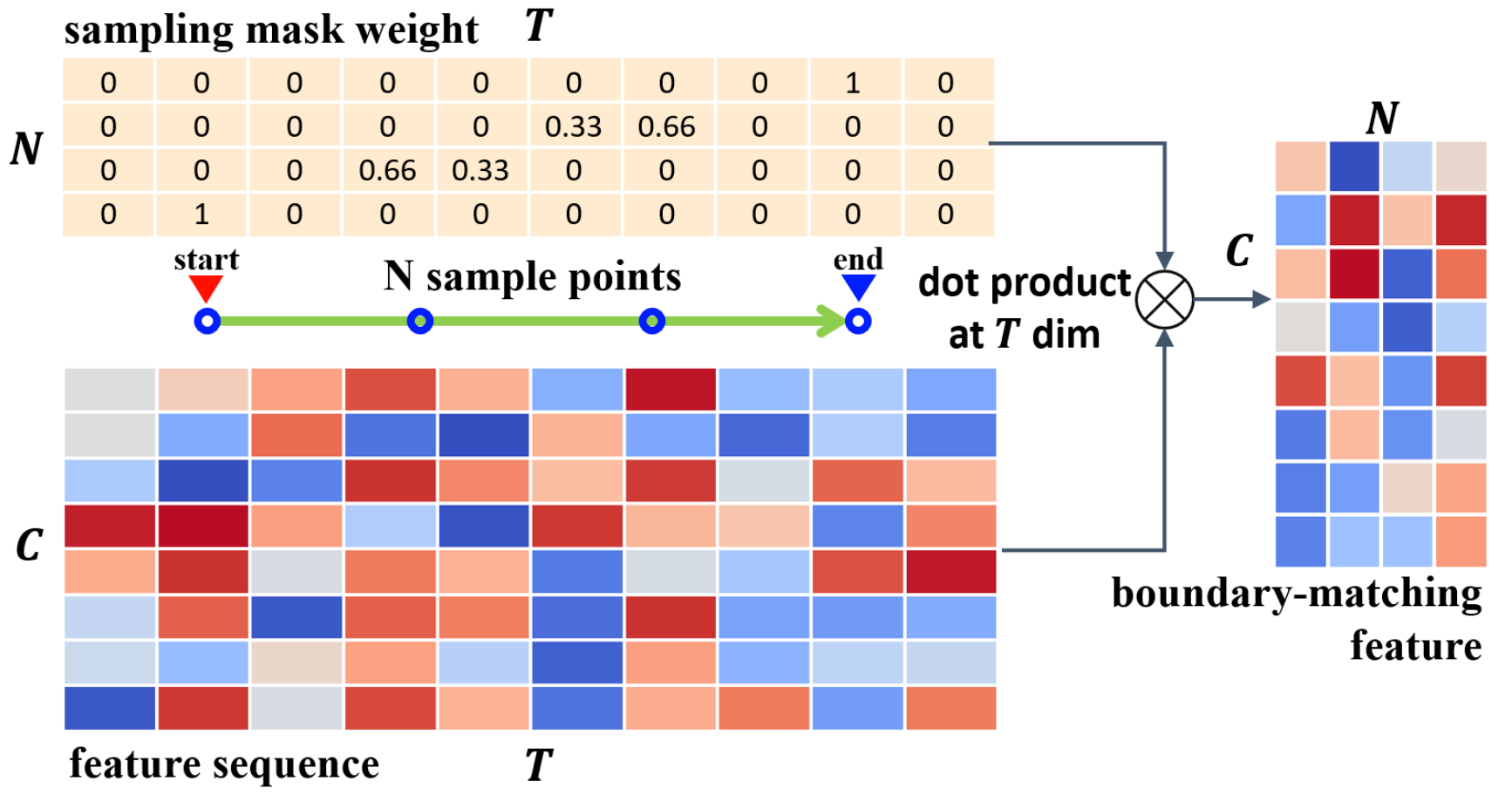
- two problems:
- how to sample feature in non-integer point:
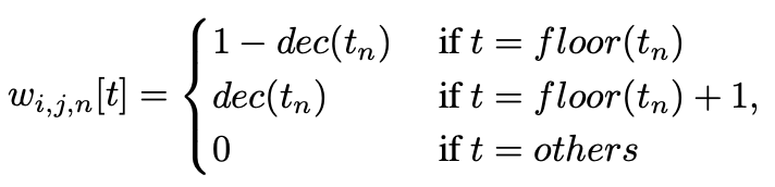
- how to sample feature for all proposals simultaneously:
- expanding $w_{i,j} ∈ R^{N ×T}$ to $W ∈ R^{N ×T ×D×T}$ for all proposals in BM confidence map.
- get $MF ∈ R^{C×N×D×T}$ by using dot product: $S{F} ∈ R^{C×T}$ and $W^T ∈ R^{T×N×D×T}$. ($W$ can be pre-generated because it’s the same for different videos, the inference speed of BM layer is very fast. Is T is the same for the different videos? Ans: BMN#Base module|Base module and BMN#Training of BMN#Training Data Construction|Training Data Construction. TODO: review code)
- how to sample feature in non-integer point:
Base module
- adopt a long observation window with length $l_ω$ to truncate the untrimmed feature sequence with length $l_f$ .
- So here $lw$ is $T$ in $S{F} ∈ R^{C×T}$.
Proposal Evaluation Module(PEM)
- Final generate: $MC\in R^{D×T}$, but there are two predicted $M_C$: $M{CC}$, $M_{CR}$, being trained using binary classification and regression loss function separately. TODO: review code.
Training of BMN
TEM vs PEM:
- TEM: learns local boundary.
- PEM: pattern global proposal context.
Training Data Construction:
- firstly, extract all feature sequence F with length.
- get many observation windows with length $l_w$ with 50% overlap.
- here every window contains at least one ground-truth action instance.
Label Assignment
TEM
- denote its starting and ending regions as $r_S = [t_s − d_g /10, t_s +d_g/10]$ and $r_E =[t_e−d_g/10,t_e+d_g/10]$separately.
- denote its local region as $r{t_n} = [t_n −d_f /2, t_n +d_f /2]$, where $d_f = t_n −t{n−1}$ is the temporal interval between two locations.
- Then calculate overlap ratio IoR of $r{t_n}$ with $r_S$ and $r_E$ separately, and denote maximum IoR as $g^s{tn}$ and $g^e{t_n}$ separately.
- here IoR is defined as the overlap ratio with ground-truth proportional to the duration of this region. TODO: code review.
- Thus generate $G{S,ω}={g^s{tn}}^{l_w}{n=1}$ and $G{E,ω}={g^e{tn}}^{l_w}{n=1}$ as label of TEM.
PEM
- Purpose: BM label map $G_C ∈ R^{D×T}$.
- For a proposal $φ{i,j}=(t_s=t_j, t_e=t_j+t_i)$ , calculate its IoU with all $φ_g$ in $Ψω$, and denote the maximum IoU as $g^c{i,j}$ . Thus we can generate $G_C={g^c{i,j}}^{D,lω}{i,j=1}$ as label of PEM.
Loss
Loss of TEM
- adopt weighted binary logistic regression loss function $L{bl}$, to get the sum of starting and ending losses:$$L{TEM} =L{bl}(P_S,G_S)+L{bl}(P_E,G_E)$$
- $L{bl}(P,G)$:
$\frac{1}{l_w}\sum{i=1}^{lw}(a^+·b_i·log(p_i)+a^-·(1-b_i)·log(1-p_i))$
where $b_i = sign(g_i − θ)$ is a two-value function used to convert $g_i$ from [0, 1] to {0, 1}0, 1} based on overlap threshold$θ = 0.5$. Denoting $l^+=\sum b_i$ and $l^− = lω −l^+$, the weighted terms are $α^+ = \frac{l_w}{l^+}$ and $α^- = \frac{l_w}{l^-}$.
Loss of PEM
- Define:
$L{PEM} =L_C(M{CC},GC)+λ·L_R(M{CR},G_C)$- here $L_{bl}$ for $L_C$ , L2 loss for $L_R$ . $λ = 10$ .
- to balance the ratio between positive and negative samples in $LR$ , take all points with $g^C{i,j}>0.6$ as positive, and randomly sample $g^C_{i,j}<0.2$ as negative, ensure 1:1 for positive: negative.
Training Objective
$L=L{LEM} +λ_1 ·L{GEM} +λ_2 ·L_2(Θ)$
where $L_2(Θ)$ is L2 regularization term, $λ_1$, $λ_2$ are set to 1, 0.000 to ensure different modules are trained evenly.
Refs: